The answers to the questions Q.6–Q.10 provide examples with synthetic data. These examples aim to highlight the implication of the issue that originates the question on the data analysis (e.g., the implication of sample variability for Q.6). To this aim, the following general steps were undertaken:
We defined a directed acyclic graph (DAG), which summarises qualitatively the relationship between the variables chosen.
Following the structure of the DAG, we generate a synthetic dataset. The data-generating parameters and the functional form used for the simulation are defined by us and therefore known.
To contextualise the data analysis, we assumed an objective in terms of data analytic question type (e.g., descriptive, inferential, etc.).
Consequently, a regression analysis was performed. This analysis aimed to answer the question of interest, but we did so by correctly and incorrectly specifying the regression model, and therefore, highlighting the specific pitfall.
Code
library(ggdag)# for DAGlibrary(dagitty)library(ggplot2)# for visualisationdag_coords.left<-data.frame(name =c('T', 'C', 'S', 'V'), x =c(1, 2, 3, 2), y =c(1.2, 1.2, 1.2, 1))dag_coords.right<-data.frame(name =c('T', 'C', 'S', 'V', 'uT', 'uC', 'uS', 'uV'), x =c(1, 2, 3, 2, 1, 2, 3, 1.5), y =c(1.2, 1.2, 1.2, 1, 1.3, 1.3, 1.3, 1))dag_coords.u<-data.frame(name =c('uT', 'uC', 'uS', 'uV'), x =c(1, 2, 3, 1.5), y =c(1.3, 1.3, 1.3, 1))dagify(C~S,C~T,V~S+C+T, coords =dag_coords.left)|>ggplot(aes(x =x, y =y, xend =xend, yend =yend))+geom_dag_text(colour='black', size =8, parse =TRUE, family =c('mono'), label =c(expression(bold(C)), expression(bold(S)), expression(bold(T)), expression(bold(V))))+geom_dag_edges(arrow_directed =grid::arrow(length =grid::unit(8, 'pt'), type ='open'), family =c('mono'), fontface =c('bold'))+coord_cartesian(xlim =c(1, 3), ylim =c(1, 1.3))+theme_dag()dagify(T~uT,S~uS,C~S+T+uC,V~S+C+T+uV, coords =dag_coords.right)|>ggplot(aes(x =x, y =y, xend =xend, yend =yend))+geom_dag_text(colour='black', size=8, parse =TRUE, family =c('mono'), label =c(expression(bold(C)), expression(bold(S)), expression(bold(T)), expression(bold(V)), expression(bold(u[C])), expression(bold(u[S])), expression(bold(u[T])), expression(bold(u[V]))))+geom_point(data =dag_coords.u, mapping =aes(x =x, y =y), inherit.aes =FALSE, shape =1, size =14, stroke =0.9, color ='black')+geom_dag_edges(aes(x =x, y =y, xend =xend, yend =yend), arrow_directed =grid::arrow(length =grid::unit(8, 'pt'), type ='open'), family ='mono', fontface ='bold')+coord_cartesian(xlim =c(1, 3), ylim =c(1, 1.3))+theme_dag()
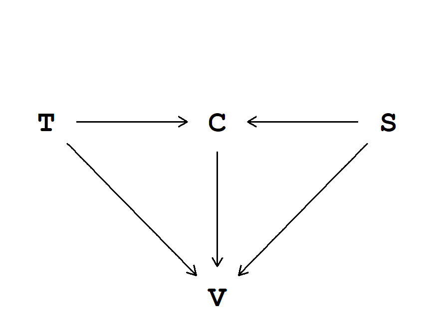
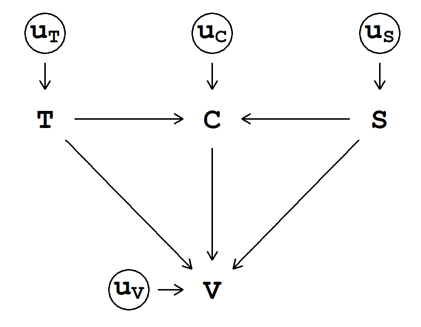
Fig. 1. Graphical representation via DAG of the data-generating process. Indoor air temperature (T) and biological sex (S) influence thermal sensation vote (V) both directly and indirectly, passing through clothing insulation (C).
All the DAGs of the examples with synthetic data (Q.6–Q.10) share a common structure that is shown in Fig. 1 (a). This structure implies that indoor air temperature \((\text{T})\) and biological sex \((\text{S})\) influence thermal sensation vote \((\text{V})\) both directly and indirectly, passing through clothing insulation \((\text{C})\). However, generally speaking, all the variables represented in a DAG will have some causes. This is shown in Fig. 1 (b). Here the causes are circled because they are considered unobserved. This structure implies that, for example, clothing insulation \((\text{C})\) is a function of indoor air temperature \((\text{T})\), sex \((\text{S})\), and some unobserved influence \((\text{u}_\text{C})\). This unobserved influence (or set of influences) can be thought of as variations around the expected value of \(\text{C}\) for each \(\text{T}\) and \(\text{S}\). However, these unobserved causes are ignorable unless shared among the variables. As such, we will omit them from the DAGs; nevertheless, it is important to remember that they are there.
It is easy to argue with this example. Should not air humidity also be included? What if sex does not influence clothing? How do you know that the chosen data-generating coefficients are appropriate? But this misses the point. In this example (and the ones that follow), we selected a few variables of interest to limit the complexity of the example itself and shift the focus to statistical data analysis. Moreover, it could be contended that if there are challenges in estimating the quantity of interest in these simple examples, it is likely that there will be more complexities associated with real-world data.
Brooks, M.E., Kristensen, K., Benthem, K.J. van, Magnusson, A., Berg, C.W., Nielsen, A., Skaug, H.J., Maechler, M., Bolker, B.M., 2017. glmmTMB: Balances speed and flexibility among packages for zero-inflated generalized linear mixed modeling. The R Journal 9, 378–400. https://doi.org/10.32614/RJ-2017-066
Bürkner, P.-C., 2018. Advanced bayesian multilevel modeling with the r package brms. The R Journal 10, 395–411. https://doi.org/10.32614/RJ-2018-017
Bürkner, P.-C., 2017. brms: An r package for bayesian multilevel models using stan. Journal of Statistical Software 80, 1–28. https://doi.org/10.18637/jss.v080.i01
Textor, J., Zander, B. van der, Gilthorpe, M.S., Liśkiewicz, M., Ellison, G.T., 2016. Robust causal inference using directed acyclic graphs: The r package "dagitty". International Journal of Epidemiology 45, 1887–1894. https://doi.org/10.1093/ije/dyw341
Wickham, H., Averick, M., Bryan, J., Chang, W., McGowan, L.D., François, R., Grolemund, G., Hayes, A., Henry, L., Hester, J., Kuhn, M., Pedersen, T.L., Miller, E., Bache, S.M., Müller, K., Ooms, J., Robinson, D., Seidel, D.P., Spinu, V., Takahashi, K., Vaughan, D., Wilke, C., Woo, K., Yutani, H., 2019. Welcome to the tidyverse. Journal of Open Source Software 4, 1686. https://doi.org/10.21105/joss.01686